Formation channels of Gravitational Waves (GWs)

This is a tutorial that can be used for live teaching/demos, it should fill about ~1hr of class

In this jupyter notebook we will walk through and re-create some of the figures from https://arxiv.org/pdf/2010.00002.pdf on Chemically Homogeneous Evolution by Jeff Riley. A PDF of this paper can be found in the directory under the name CHE_paper.pdf.

Notebook by Floor Broekgaarden, Jeff Riley and Ilya Mandel, originally created for the Saas Fee PhD School

The original data can be found on Zenodo https://zenodo.org/record/5595426 For this tutorial we have downloaded COMPAS_Output.h5 from the auhtor’s dataset. Note that this data is run with a slightly older version of COMPAS than the most recent COMPAS.

---

Throughout this notebook and in class we will use several acronyms and definitions listed below

Definitions:

• CHE: Chemically Homogeneous Evolution,

• GW: Gravitational Waves

• DCO: Double Compact Object

• BH: Black Hole

• NS: Neutron Star

• Primary: in this notebook always refers to the star that was most massive at the zero age main sequence (ZAMS)

• Secondary: in this notebook always refers to the star that was least massive at the zero age main sequence (ZAMS)

• ZAMS: Zero Age Main Sequence: this is in COMPAS where stars start their lives.

# first we will import some of the packages that we will use
import h5py as h5
import numpy as np
import os
import matplotlib.pyplot as plt

# we will use astropy for some useful constants and units
from astropy import units as u
from astropy import constants as const
from matplotlib.ticker import (FormatStrFormatter,
                               AutoMinorLocator)
from IPython.display import Image # to open images in Ipython

# add path to where the COMPASOutput.h5 file is stored.
# For you the part '~/Downloads/' is probably different
path = '/Users/floorbroekgaarden/Downloads/COMPAS_Output.h5' # change this line!

# the following line reads in the data
fdata = h5.File(path, 'r')
list(fdata.keys())  # print the different files within the hdf5 folder:



# to close the file you will have to use fdata.close()

['CommonEnvelopes', 'DoubleCompactObjects', 'Supernovae', 'SystemParameters']

the files above ‘DoubleCompactObjects’, ‘Supernovae’, ‘SystemParameters’ store the properties of the simulated binaries at the stages of the ‘commen enevelope’ (in case there is one), the moment of double object formation, the moment of the supernova, and the initial conditions (at the zero-age main sequence).

We can view what parameters are stored by again using the command .keys()

print(list(fdata['DoubleCompactObjects'].keys()))

print()

print(list(fdata['SystemParameters'].keys()))

print()

print(list(fdata['Supernovae'].keys()))

['Coalescence_Time', 'Eccentricity@DCO', 'MT_Case_1', 'MT_Case_2', 'Mass_1', 'Mass_2', 'Merges_Hubble_Time', 'Recycled_NS_1', 'Recycled_NS_2', 'SEED', 'Separation@DCO', 'Stellar_Type_1', 'Stellar_Type_2', 'Time']

['CE_Alpha', 'CH_on_MS_1', 'CH_on_MS_2', 'Eccentricity@ZAMS', 'Equilibrated', 'Equilibrated_At_Birth', 'Error', 'Experienced_RLOF_1', 'Experienced_RLOF_2', 'Experienced_SN_Type_1', 'Experienced_SN_Type_2', 'LBV_Multiplier', 'LBV_Phase_Flag_1', 'LBV_Phase_Flag_2', 'Mass@ZAMS_1', 'Mass@ZAMS_2', 'Merger', 'Merger_At_Birth', 'Metallicity@ZAMS_1', 'Metallicity@ZAMS_2', 'Omega@ZAMS_1', 'Omega@ZAMS_2', 'SEED', 'SN_Kick_Magnitude_Random_Number_1', 'SN_Kick_Magnitude_Random_Number_2', 'SN_Kick_Mean_Anomaly_1', 'SN_Kick_Mean_Anomaly_2', 'SN_Kick_Phi_1', 'SN_Kick_Phi_2', 'SN_Kick_Theta_1', 'SN_Kick_Theta_2', 'Separation@ZAMS', 'Sigma_Kick_CCSN_BH', 'Sigma_Kick_CCSN_NS', 'Sigma_Kick_ECSN', 'Sigma_Kick_USSN', 'Stellar_Type@ZAMS_1', 'Stellar_Type@ZAMS_2', 'Stellar_Type_1', 'Stellar_Type_2', 'Time', 'Unbound', 'WR_Multiplier']

['Applied_Kick_Velocity_SN', 'Drawn_Kick_Velocity_SN', 'Eccentricity', 'Eccentricity<SN', 'Experienced_RLOF_SN', 'Fallback_Fraction_SN', 'Hydrogen_Poor_SN', 'Hydrogen_Rich_SN', 'Kick_Velocity(uK)', 'Mass_CO_Core@CO_SN', 'Mass_CP', 'Mass_Core@CO_SN', 'Mass_He_Core@CO_SN', 'Mass_SN', 'Mass_Total@CO_SN', 'Orb_Velocity<SN', 'Runaway_CP', 'SEED', 'SN_Kick_Phi_SN', 'SN_Kick_Theta_SN', 'SN_Type_SN', 'Separation', 'Separation<SN', 'Stellar_Type_Prev_CP', 'Stellar_Type_Prev_SN', 'Stellar_Type_SN', 'Supernova_State', 'Systemic_Velocity', 'Time', 'True_Anomaly(psi)_SN', 'Unbound']

The meaning of all parameters and files are described here https://compas.readthedocs.io/en/latest/pages/User%20guide/COMPAS%20output/standard-logfiles.html

Now that we have the data, we can do some data investigation. Here is an example of how to read the “SEED” parameter, which is a unique number for each binary that is run.

SEED_DCO = fdata['DoubleCompactObjects']["SEED"][...].squeeze()
print(SEED_DCO)

[  400047   400065   400101 ... 11599854 11599926 11599965]

Question 1

• a: check and write down the number of rows (entries) of each of the dataset groups, ‘DoubleCompactObjects’, ‘Supernovae’, ‘SystemParameters’.

---

• b: If the lengths of the rows are different why is this so? And does it make sense which group has the most/least rows?

---

Hint: you might want to look at table 1 in the paper CHE_paper.pdf and the descriptions at https://compas.readthedocs.io/en/latest/pages/User%20guide/COMPAS%20output/standard-logfiles.html

• c: Why is the number of rows in ‘DoubleCompactObjects’ not the same as the total number of ‘BBHs formed’ in Table 1 from this paper?

---

Answer 1:

Below are a few methods shown to print the number of rows (but there are many ways to do this). We find that DoubleCompactObjects has 291253 rows, SystemParameters has 12000000 number of rows and the group Supernovae has 6213168 number of rows.

• The systemparameters is easiest to understand: this file prints one line (row) for each binary that the author simulated in COMPAS. You can read in the paper or see in Table 1 (under “Number of binaries evolved” and then the “total” column) that this is exactly 12 million. Which is indeed the same as the number of rows in the dataset.

• Second we have the group ‘DoubleCompactObjects’, this is the dataset that prints the properties at the moment a double compact object binary (DCO) is formed. This is a rare occurance in our simulations (even if we only model massive stars). And so the number of rows/entries in this file is much much smaller and reduced to only 291253 (almost 300 000) which is the outcome of about ~2.4% of the all simulated systems. You can see that this number is close to, but slightly larger than the 261,741 “Total” BBHs formed in Table 1 of the paper. This is because the ‘DoubleCompactObjects’ file also contains NS+NS and BH+NS mergers on top of the BH+BH mergers, whereas the table only quotes the number of BH+BH mergers residing in the data.

• Last, the ‘Supernovae’ file prints the properties of the binary whenever in the simulation a supernova occurs. This is a tricky one to explain. There are 2 supernova that occur to form a DCO system, so you expect this file to always be larger than 2x the double compact object file. On the other hand, of the stars that do not form a DCO system, many either merge as stars, or disrupt during the first SN, in which case the simulation stops following the evolution of the binary and future SNe are not printed.

# Method 1, based on the example above


# all three groups contain the parameter "SEED", so we can use this to print the lengths
for group in ['DoubleCompactObjects', 'SystemParameters', 'Supernovae']:
    SEED = fdata[group]["SEED"][...].squeeze()
    print('group %s has %s number of rows'%(group, len(SEED)))

group DoubleCompactObjects has 291253 number of rows
group SystemParameters has 12000000 number of rows
group Supernovae has 6213168 number of rows

# Method 2: Or even shorter:

# all three groups contain the parameter "SEED", so we can use this to print the lengths
for group in ['DoubleCompactObjects', 'SystemParameters', 'Supernovae']:
    print('group %s has %s number of rows'%(group, fdata[group]["SEED"].len()))

group DoubleCompactObjects has 291253 number of rows
group SystemParameters has 12000000 number of rows
group Supernovae has 6213168 number of rows

# Method 3, writing everything out:

lenDCO = len(fdata['DoubleCompactObjects']['SEED'][...].squeeze())
print('group DoubleCompactObjects has %s number of rows'%lenDCO)

lenSys = len(fdata['SystemParameters']['SEED'][...].squeeze())
print('group SystemParameters has %s number of rows'%lenSys)

lenSNe = len(fdata['Supernovae']['SEED'][...].squeeze())
print('group Supernovae has %s number of rows'%lenSNe)

group DoubleCompactObjects has 291253 number of rows
group SystemParameters has 12000000 number of rows
group Supernovae has 6213168 number of rows

Example 1: plotting BH masses

---

below we show an example of how to obtain and plot the compact object masses in the dataset

# this is just a little function that we will use to make the plot more beautiful (bigger ticks, labels)
# However, you do not have to use this (just uncommoment "layoutAxes" everywhere)

def layoutAxes(ax, nameX='', nameY='', \
               labelSizeMajor = 10, fontsize = 25, second=False, labelpad=None, setMinor=True):
    """
    Tiny code to do the layout for axes in matplotlib
    """
    tickLengthMajor = 10
    tickLengthMinor = 5
    tickWidthMajor  = 1.5
    tickWidthMinor  = 1.5

    #rc('axes', linewidth=2)
    #label1 always refers to first axis not the twin
    if not second:
        for tick in ax.xaxis.get_major_ticks():
            tick.label1.set_fontsize(fontsize)
            #tick.label1.set_fontweight('bold')
        for tick in ax.yaxis.get_major_ticks():
            tick.label1.set_fontsize(fontsize)
            #tick.label1.set_fontweight('bold')
    if second:
        for tick in ax.xaxis.get_major_ticks():
            tick.label2.set_fontsize(fontsize)
            #tick.label1.set_fontweight('bold')
        for tick in ax.yaxis.get_major_ticks():
            tick.label2.set_fontsize(fontsize)
            #tick.label1.set_fontweight('bold')
    for axis in ['top','bottom','left','right']:
        ax.spines[axis].set_linewidth(1.2)
    ax.tick_params(length=tickLengthMajor, width=tickWidthMajor, which='major')
    ax.tick_params(length=tickLengthMinor, width=tickWidthMinor, which='minor')
    ax.set_xlabel(nameX, fontsize=fontsize,labelpad=labelpad)#,fontweight='bold')
    ax.set_ylabel(nameY, fontsize=fontsize,labelpad=labelpad)#, fontweight='bold')

    if setMinor==True:
        # add minor ticks:
        ax.xaxis.set_minor_locator(AutoMinorLocator())
        ax.yaxis.set_minor_locator(AutoMinorLocator())

    return ax

fDCO      = fdata['DoubleCompactObjects']


M1 =  fDCO['Mass_1'][...].squeeze()  # mass in Msun of the compact object resulting from the *primary star*
M2 =  fDCO['Mass_2'][...].squeeze()  # mass in Msun of the compact object resulting from the *secondary star*

f, ax= plt.subplots(1, 1,  figsize=(10,10))

plt.scatter(M1, M2)
plt.xlabel('Mass of compact object from primary star [Msun]', fontsize=20)
plt.ylabel('Mass of compact object from secondary star [Msun]', fontsize=20)
plt.show()

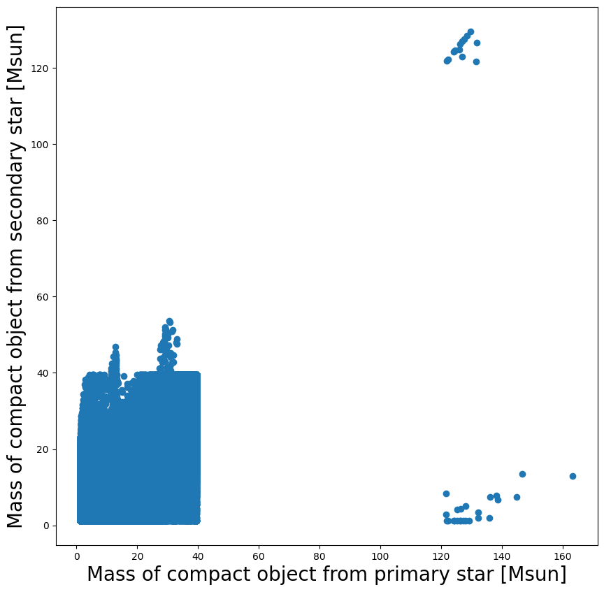
Question 2:

• a): can you explain some of the features in the plot above? E.g., where are the gaps, where are the most datapoints?

• b): Are there any BH+NS or NS+NS in the dataset? If so, plot them

• c): extra: how many BH+NS, vs. NS+NS vs. BH-BH systems are there? And what is the total?

Hint: A NS in this COMPAS simulation is defined as a compact object with mass < 2.5 Msun

We first plot the NS-NS, NS-BH and BH-BH DCO systems in seperate plots below.

For this we use the definition that a NS in COMPAS is always below < 2.5 Msun, and that this value thus indicates the boundary between NSs and BHs. This does not have to be true in nature (nature might actually have a slightly different value for this boundary, for which a lot of active research is being conducted).

There are also many other ways to do this, including checking for the StellarType of the stars.

f, ax= plt.subplots(1, 1,  figsize=(10,10))

mask_M1isNS = (M1 <= 2.5) # M1 is a NS if mass is <= 2.5 Msun
mask_M2isNS = (M2 <= 2.5) # M2 is a NS if mass is <= 2.5 Msun

mask_NSNS = ((mask_M1isNS==1) & (mask_M2isNS==1))

plt.scatter(M1[mask_NSNS], M2[mask_NSNS], c='darkgreen', label='NS+NS')


layoutAxes(ax=ax, nameX='Mass of compact object from primary star [Msun]',\
           nameY='Mass of compact object from secondary star [Msun]')

plt.legend(fontsize=20)
plt.show()

print('The total number of NS+NS systems in the dataset is %s'%len(M1[mask_NSNS]))

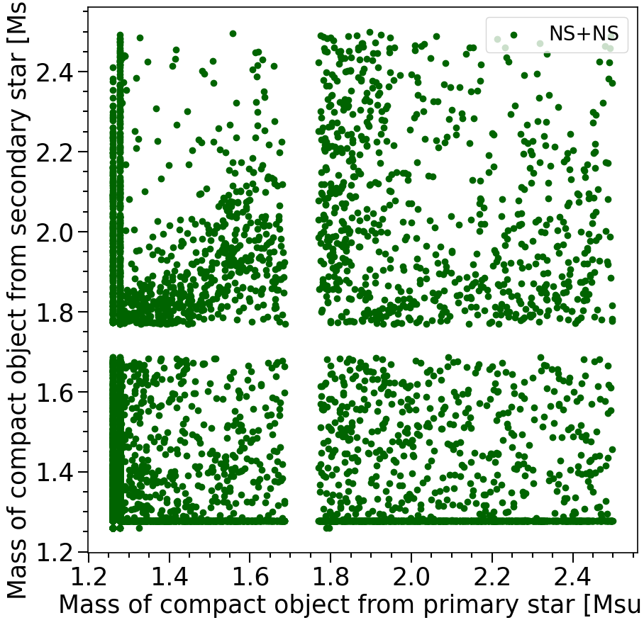
The total number of NS+NS systems in the dataset is 11248

Features in the plot above:

In the plot above we see that the NS-NS systems formed in COMPAS have masses between 1.2-2.5 solar masses. This is the neutron star mass range that is expected from the NS equation of state.

I don’t expect that most students will know this: There is a gap around 1.7 Msun. But this is an artifact from the SN remnant mass prescription used in COMPAS There is a little bit of a pile up of NS systems around 1.25 solar masses. These systems come from electron capture supernovae and ultra-stripped supernovae.

f, ax= plt.subplots(1, 1,  figsize=(10,10))
mask_M1isNS = (M1 <= 2.5) # M1 is a NS if mass is <= 2.5 Msun
mask_M2isNS = (M2 <= 2.5) # M2 is a NS if mass is <= 2.5 Msun


mask_NSBH = ((mask_M1isNS==1) & (mask_M2isNS==0)) | ((mask_M1isNS==0) & (mask_M2isNS==1))


plt.scatter(M1[mask_NSBH], M2[mask_NSBH], c='orange', label='NS+BH')

layoutAxes(ax=ax, nameX='Mass of compact object from primary star [Msun]',\
           nameY='Mass of compact object from secondary star [Msun]')
plt.legend(fontsize=20)
plt.show()

print('The total number of BH+NS systems in the dataset is %s'%len(M1[mask_NSBH]))

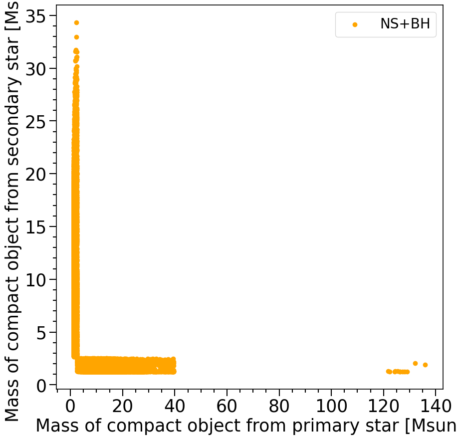
The total number of BH+NS systems in the dataset is 19383

Features in the plot above:

In the plot above we see that the BH-NS systems formed in COMPAS have NS masses between 1.2-2.5 solar masses. This is the neutron star mass range that is expected from the NS equation of state. The BHs are typically between 2.5 and 40 solar masses (but some extreme cases exist, but do not trust these too much).

The gap between 40 and ~120 solar masses where no BHs form is a result from the pair-instability SN remnant mass gap. Where it is predicted that the Helium cores that form the BHs with masses in this gap undergo pair-instabillity and completely explode, not leaving behind any remnant.

# now the BH-BH systems:

f, ax= plt.subplots(1, 1,  figsize=(10,10))

mask_M1isNS = (M1 < 2.5) # M1 is a NS if mass is <= 2.5 Msun
mask_M2isNS = (M2 < 2.5) # M2 is a NS if mass is <= 2.5 Msun


Stellar_Type_1 = fDCO['Stellar_Type_1'][...].squeeze()
Stellar_Type_2 = fDCO['Stellar_Type_2'][...].squeeze()



mask_BHBH = ((mask_M1isNS==0) & (mask_M2isNS==0))


plt.scatter(M1[mask_BHBH], M2[mask_BHBH], c='blue', label='BH+BH')

layoutAxes(ax=ax, nameX='Mass of compact object from primary star [Msun]',\
           nameY='Mass of compact object from secondary star [Msun]')
plt.legend(fontsize=20)
plt.show()

print('The total number of BH+BH systems in the dataset is %s'%len(M1[mask_BHBH]))

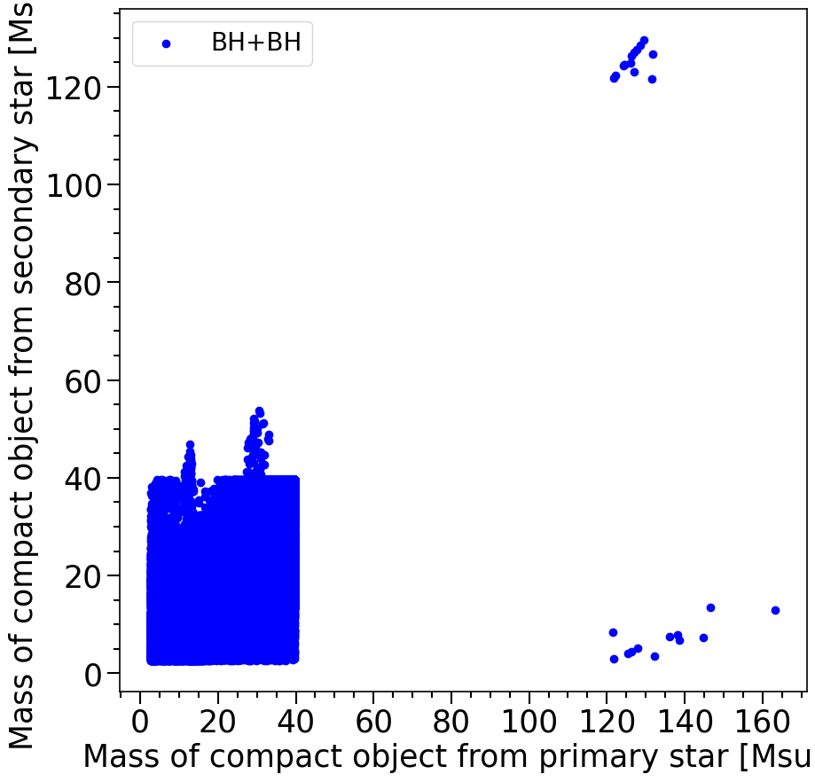
The total number of BH+BH systems in the dataset is 260622

Features in the plot above:

In the plot above we see that the BH-NS systems formed in COMPAS have NS masses between 1.2-2.5 solar masses. This is the neutron star mass range that is expected from the NS equation of state. The BHs are typically between 2.5 and 40 solar masses (but some extreme cases exist, but do not trust these too much).

The gap between 40 and ~120 solar masses where no BHs form is a result from the pair-instability SN remnant mass gap. Where it is predicted that the Helium cores that form the BHs with masses in this gap undergo pair-instabillity and completely explode, not leaving behind any remnant.

There is a couple of interesting things to note:

First of all the number of DCO systems are: BHBH: 260622 BHNS: 19383 NSNS: 11248

BHBH are most common in te simulation, but that is partly due to the systems that have been evolved in COMPAS and the low metallicities.

There are systems that undergo “mass ratio reversal”, these are systems where the mass of the compact object from the secondary star at ZAMS (initially least massive star) ends up forming the most massive BH in the BBH system (top left systems). These systems have “reversed” the mass ratio at some point in their evolution (during one of the mass transfer phases).

Question 3:

• a): Using the parameters in the ‘DoubleCompactObjects’ dataset and the example above, try to make a scatter plot of Total Mass (M1+M2) versus orbital Period of the BBH systems that merge within a Hubble time (13.7 Gyr)

  Plot the period on the y-axis and the total mass on the x-axis. Plot the period in days.

Hint: You might want to use Kerpler’s III law to complete the function below

Hint: you will have to select BH+BH systems, and only systems that merge within a Hubble time

def separation_to_period_circular_case(separation=10*u.AU, M1=1*u.M_sun, M2=1*u.M_sun):
    """calculate Period from separation
    separation is separation of the binary (needs to be given in astropy units)
    M1 and M2 are masses of the binary
    This is based on Kepler's law, using a circular orbit

    """
    G = const.G # [g cm s^2]

    ## use Kepler;s III law to calculate the period here



    ###

    return period

See the function below

def separation_to_period_circular_case(separation=10*u.AU, M1=1*u.M_sun, M2=1*u.M_sun):
    """calculate Period from separation
    separation is separation of the binary (needs to be given in astropy units)
    M1 and M2 are masses of the binary
    This is based on Kepler's law, using a circular orbit

    """
    G = const.G # [g cm s^2]


    mu = G*(M1+M2)
    period = 2*np.pi * np.sqrt(separation**3/mu)

    return period

mask_M1isNS = (M1 <= 2.5) # M1 is a NS if mass is <= 2.5 Msun
mask_M2isNS = (M2 <= 2.5) # M2 is a NS if mass is <= 2.5 Msun
mask_BHBH = ((mask_M1isNS==0) & (mask_M2isNS==0))  # if true then the system is a BHBH

separation =  fDCO['Separation@DCO'][...].squeeze() # in AU
Period = separation_to_period_circular_case(separation*u.au, M1*u.M_sun, M2*u.M_sun)
# the merger time is called the "coalescence time"
coalescence_time =  fDCO['Coalescence_Time'][...].squeeze() * u.Myr # Myr
t_Hubble = 13.7 *u.Gyr
mask_tHubble = (coalescence_time < t_Hubble)

mask_systemsOfInterest = (mask_BHBH==1) & (mask_tHubble==1)


f, ax= plt.subplots(1, 1,  figsize=(10,10))

plt.scatter((M1+M2)[mask_systemsOfInterest], Period[mask_systemsOfInterest].to(u.d))

xlabel = 'Total BBH Mass [Msun]'
ylabel = 'Period [day]'
layoutAxes(ax=ax, nameX=xlabel,nameY=ylabel)
plt.yscale('log')

plt.show()

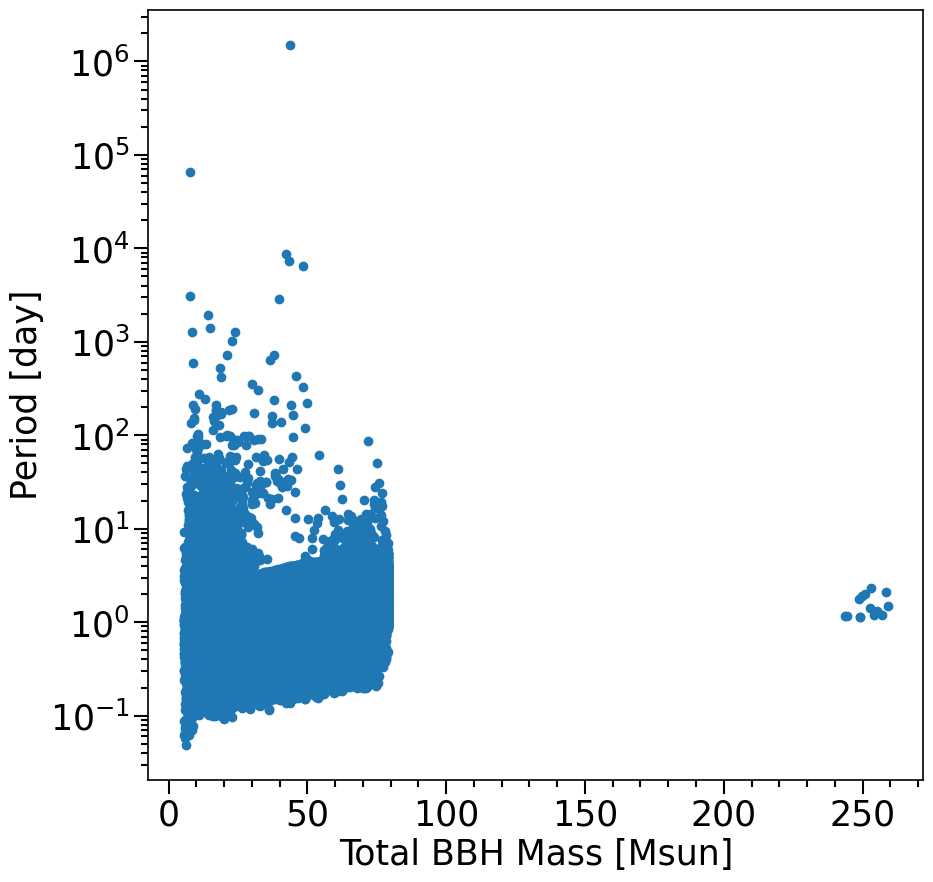
• a): Why does the plot that you created look different compared to the figure 6 in https://arxiv.org/pdf/2010.00002.pdf? (you may ignore the metallicity axes)

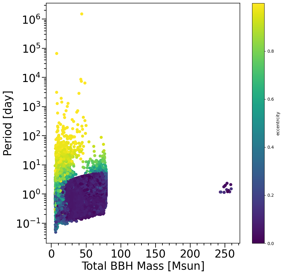
• b): There is a tail of systems at rather large orbital periods that are merging. How is this possible?

Hint 4b: plot the eccentricity as a color gradient on the marker using the “c=” option of plt.scatter. How is eccentricity imparted to these systems?

Possible answers: Figure 6 only shows the data for one of the submodels (f_WR=.2) and only shows the CHE systems, and the axes are in log.

ecc = fDCO['Eccentricity@DCO'][...].squeeze()


f, ax= plt.subplots(1, 1,  figsize=(10,10))

plt.scatter((M1+M2)[mask_systemsOfInterest], Period[mask_systemsOfInterest].to(u.d), c=ecc[mask_systemsOfInterest])

xlabel = 'Total BBH Mass [Msun]'
ylabel = 'Period [day]'
layoutAxes(ax=ax, nameX=xlabel,nameY=ylabel)
plt.yscale('log')
plt.colorbar(label='eccentrcity')

plt.show()

For binaries, Stellar_Type@ZAMS(1) and Stellar_Type@ZAMS(2) will tell you the initial stellar type of each star - type 16 is CH. CH_on_MS(1) and CH_on_MS(2) are each true if the star remained as CH for the entire MS - they will be false if the star spun down and stopped being CH on the MS. So any star that was initially CH, and stayed CH on the entire MS is considered to be CHE. We can check which of our binary black holes is a “CHE” by using this information stored in the ‘systemParameters’ file, and matching it with the double compact object files using the randomSeed.

Note that we also have to remove binaries that merged on the ZAMS as stars, since we are not interested in these

fsys      = fdata['SystemParameters']

CH_on_MS_1 =  fsys['CH_on_MS_1'][...].squeeze()  # mass in Msun of the compact object resulting from the primary
CH_on_MS_2 =  fsys['CH_on_MS_2'][...].squeeze()  # mass in Msun of the compact object resulting from the secondary
Stellar_TypeZAMS_1  =  fsys['Stellar_Type@ZAMS_1'][...].squeeze()  # mass in Msun of the compact object resulting from the primary
Stellar_TypeZAMS_2  =  fsys['Stellar_Type@ZAMS_2'][...].squeeze()  # mass in Msun of the compact object resulting from the secondary

# binaries that merge at birth as stars
Merger_At_Birth = fsys['Merger_At_Birth'][...].squeeze()

# SEED of the system Parameters (unique number corresponding to each binary)
SEED = fsys['SEED'][...].squeeze()  # mass in Msun of the compact object resulting from the secondary

# the CHE systems are then selected by systems that are CHE on ZAMS (stellar type 16) AND remain CHE on the MS (main sequence)
# in addition we do not want systems that Merged at Birth
mask_CHE =  (CH_on_MS_1==1) & (CH_on_MS_2==1) & (Stellar_TypeZAMS_1==16) &  (Stellar_TypeZAMS_2==16) & (Merger_At_Birth==0)

print(np.sum(mask_CHE), 'are CHE out of ', len(mask_CHE), 'systems run')


# let's find the seed of the CHE systems:
SEED_CHE = SEED[mask_CHE]
print(SEED_CHE)

13644 are CHE out of  12000000 systems run
[  400378   400412   402049 ... 11589507 11589863 11594670]

We find 13644 total CHE binaries in our simulation, note that this is the same as the number quoted in the CHE paper under “Both stars remained on the CH” and “Total” in Table 1

• a): Using the code above, recreate figure 6 in https://arxiv.org/pdf/2010.00002.pdf? (you may ignore the metallicity axes)

• b): Explain what you see

Hint: A useful line of code is: np.in1d(), below is an example of how it works

# example of np.in1d() function

A = [1,2,3]
B = [1,3,5,7,9]

print(np.in1d(A, B))

[ True False  True]

Answer 5

mask_M1isNS = (M1 <= 2.5) # M1 is a NS if mass is <= 2.5 Msun
mask_M2isNS = (M2 <= 2.5) # M2 is a NS if mass is <= 2.5 Msun
mask_BHBH = ((mask_M1isNS==0) & (mask_M2isNS==0))  # if true then the system is a BHBH

separation =  fDCO['Separation@DCO'][...].squeeze() # in AU
Period = separation_to_period_circular_case(separation*u.au, M1*u.M_sun, M2*u.M_sun)
# the merger time is called the "coalescence time"
coalescence_time =  fDCO['Coalescence_Time'][...].squeeze() * u.Myr # Myr
t_Hubble = 13.7 *u.Gyr
mask_tHubble = (coalescence_time < t_Hubble)

# this is the parameter that describes the Wolf Rayet factor f_WR that was used.
WR_Multiplier = fsys['WR_Multiplier'][...].squeeze()

# mask BBHs that merge in a Hubble time
mask_systemsOfInterest = (mask_BHBH==1) & (mask_tHubble==1)

# add the mask of systems that are CHE. Since the CHE mask is based on systemParameters we have
# to match the systems from systemParameters that we want to mask with the DCO systems, we can do this using the SEED
# a system in systemParameters will have the same SEED in DoubleCompactObjects, if it exists in both
mask_DCO_that_are_CHE = np.in1d(SEED_DCO, SEED_CHE)
mask_DCO_that_are_BBH_and_CHE = (mask_DCO_that_are_CHE ==1) & (mask_systemsOfInterest==1)

# we can mask for the f_WR = 0.2 factor that is used in Figure 6 of the paper.
mask_fWR_02 = (WR_Multiplier==0.2)
SEED_fWR_02 = SEED[mask_fWR_02]
mask_DCO_that_are_fWR_02 = np.in1d(SEED_DCO, SEED_fWR_02)

# combine all the masks above
mask_DCO_that_are_BBH_and_CHE_and_fWR_02 = (mask_DCO_that_are_CHE ==1) & (mask_systemsOfInterest==1) & (mask_DCO_that_are_fWR_02==1)


# plot the systems
f, ax= plt.subplots(1, 1,  figsize=(10,10))

plt.scatter((M1+M2)[mask_DCO_that_are_BBH_and_CHE_and_fWR_02], Period[mask_DCO_that_are_BBH_and_CHE_and_fWR_02].to(u.d))

xlabel = 'Total BBH Mass [Msun]'
ylabel = 'Period [day]'
layoutAxes(ax=ax, nameX=xlabel,nameY=ylabel)
# plt.yscale('log')


plt.show()


print(len((M1+M2)[mask_DCO_that_are_BBH_and_CHE_and_fWR_02]))

2320

The plot above looks very similar to Figure 6, the only differences are that we did not add the Metallicity axis in this example. You can add this by using the property ‘Metallicity@ZAMS_1’ from the systemParameters.

In addition, our Period range plotted above (the ylim) is slightly larger then the ylim range plotted in Figure 6

Last, the total number of events 2320 is slightly different compared to Fig 6. This is a result from a small typo/error by the auhtor in the data version that is published versus the version that was used to run this specific figure

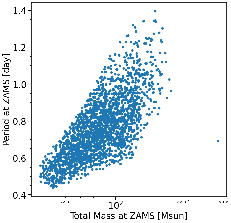
Question 6:

• a): Try to recreeat the figure 4 in https://arxiv.org/pdf/2010.00002.pdf?

• b): Explain what you see

Answer 6

See the code below. The method is very similar to the Answer to question 5, but now we have to get the ZAMS properties through the systemParameters file. For which we have to use the np.in1d again to match the datapoints

mask_M1isNS = (M1 <= 2.5) # M1 is a NS if mass is <= 2.5 Msun
mask_M2isNS = (M2 <= 2.5) # M2 is a NS if mass is <= 2.5 Msun
mask_BHBH = ((mask_M1isNS==0) & (mask_M2isNS==0))  # if true then the system is a BHBH




M1ZAMS =  fsys['Mass@ZAMS_1'][...].squeeze()  # mass in Msun of the compact object resulting from the *primary star*
M2ZAMS =  fsys['Mass@ZAMS_2'][...].squeeze()  # mass in Msun of the compact object resulting from the *secondary star*


# the separation At ZAMS is given by
separationZAMS = fsys['Separation@ZAMS'][()]
PeriodZAMS = separation_to_period_circular_case(separationZAMS*u.au, M1ZAMS*u.M_sun, M2ZAMS*u.M_sun)

# the merger time is called the "coalescence time"
coalescence_time =  fDCO['Coalescence_Time'][...].squeeze() * u.Myr # Myr
t_Hubble = 13.7 *u.Gyr
mask_tHubble = (coalescence_time < t_Hubble)

# this is the parameter that describes the Wolf Rayet factor f_WR that was used.
WR_Multiplier = fsys['WR_Multiplier'][...].squeeze()

# mask BBHs that merge in a Hubble time
mask_systemsOfInterest = (mask_BHBH==1) & (mask_tHubble==1)

# add the mask of systems that are CHE. Since the CHE mask is based on systemParameters we have
# to match the systems from systemParameters that we want to mask with the DCO systems, we can do this using the SEED
# a system in systemParameters will have the same SEED in DoubleCompactObjects, if it exists in both
mask_DCO_that_are_CHE = np.in1d(SEED_DCO, SEED_CHE)
mask_DCO_that_are_BBH_and_CHE = (mask_DCO_that_are_CHE ==1) & (mask_systemsOfInterest==1)

# we can mask for the f_WR = 1 factor that is used in Figure 4 of the paper.
mask_fWR_1 = (WR_Multiplier==1)
SEED_fWR_1 = SEED[mask_fWR_1]
mask_DCO_that_are_fWR_1 = np.in1d(SEED_DCO, SEED_fWR_1)

# combine all the masks above
mask_DCO_that_are_BBH_and_CHE_and_fWR_1 = (mask_DCO_that_are_CHE ==1) & (mask_systemsOfInterest==1) & (mask_DCO_that_are_fWR_1==1)

mask_Fig4 = np.in1d(SEED, SEED_DCO[mask_DCO_that_are_BBH_and_CHE_and_fWR_1])




# plot the systems
f, ax= plt.subplots(1, 1,  figsize=(10,10))

plt.scatter((M1ZAMS+M2ZAMS)[mask_Fig4], PeriodZAMS[mask_Fig4].to(u.d))

xlabel = 'Total Mass at ZAMS [Msun]'
ylabel = 'Period at ZAMS [day]'
layoutAxes(ax=ax, nameX=xlabel,nameY=ylabel)
plt.xscale('log')


plt.show()


print(len((M1+M2)[mask_DCO_that_are_BBH_and_CHE_and_fWR_02]))

2320

For the last part of this excersize we will use the code ‘FastCosmicIntegrator’. Our goal will be to calculate the merger rate for BBHs, so that we can compare to the analytical estimate we made earlier on.

Question 7:

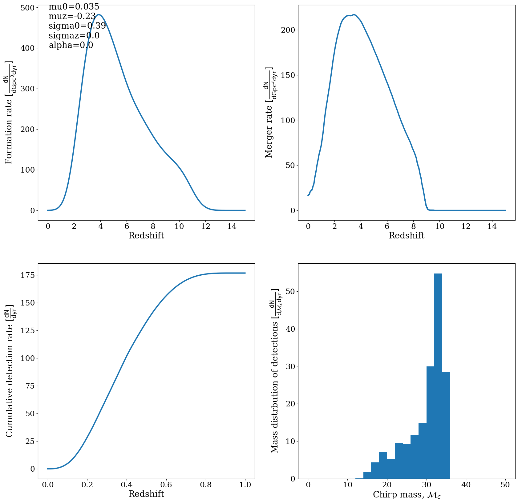
Using the code below, plot the merger rate of CHE BBHs as a function of redshift. You should at the end of running this code create a plot with four panels that show the properties of the CHE binaries

• 1. what do the panels show? What are the differences between the panels?

• b): please write down the local (z=0) BBH merger rate, and compare this with your analytically calculated rate

• c): compare both rates with the other BBH rates as reported in Mandel & Broekgaarden et al. (2021) (Fig 3)

• d): Repeat the excersize above, and answer 7a & 7b above, but now for all BBHs (including non CHE). You can do this by changing dco_type to ‘BBH’. What are the differences

Hint we can do an approximate calculation by combining the Wolf Rayet factors. If you want to do the more expert version you can modify the code in ClassCOMPAS (setCOMPASDCOmask) and add the mask of a specific f_WR factor

# change the line to point to your path

!python3 FastCosmicIntegration.py \
--dco_type 'CHE_BBH' \
--path '/Users/floorbroekgaarden/Downloads/COMPAS_Output.h5' \
--maxz 15 \
--dontAppend

/Library/Frameworks/Python.framework/Versions/3.11/Resources/Python.app/Contents/MacOS/Python: can't open file '/Users/floorbroekgaarden/Projects/GitHub/COMPAS/utils/Tutorial/Tutorial_reproduce_CHE_paper_teaching_demo_example/FastCosmicIntegration.py': [Errno 2] No such file or directory

!ls

CHE_evolution_demo.ipynb
CHE_evolution_demo_ANSWERS.ipynb
COMPAS_Documentation.pdf
Rate_Infomu00.035_muz-0.23_alpha0.0_sigma00.39_sigmaz0.0.png
SNR_Grid_IMRPhenomPv2_FD_all_noise.hdf5
__pycache__
old_ClassCOMPAS.py
old_FastCosmicIntegration.py
old_selection_effects.py
old_totalMassEvolvedPerZ.py

# show the image in the notebook:
Image(filename='./Rate_Infomu00.035_muz-0.23_alpha0.0_sigma00.39_sigmaz0.0.png')

Answer 7

The rates for CHE around redshift 0 are about 20 Gpc^-3 yr^-1 for the mixture model (note that we have to select either of the Wolf Rayet factors if we want to get an absolute rate for one fixed model. ) This is indeed about the mean of the Rates quoted by Riley +2021, and corresponds to the CHE rates as shown in Fig 3 of Mandel & Broekgaarden

The CHE rates are somewhat lower compared to the isolated binary evoluton rates, and many of the other channel rates. This is because the CHE channel is a rare channel: you need very specific intitial conditions (masses, metallicities) to form CHE stars.

Extra Question 8:

Play around with some of the parameters in the code FastCosmicIntegrater, do the rates go up or down? Is this expected?

Answer 8

Doing this for ‘BBH’ should give you a rate of about 100 Gpc^-3 yr^-1 which is right on the ballpark of the observations

!python3 FastCosmicIntegration.py \
--dco_type 'BBH' \
--path '../../data/COMPAS_Output_reduced.h5' \
--maxz 15 \
--dontAppend

/Library/Frameworks/Python.framework/Versions/3.11/Resources/Python.app/Contents/MacOS/Python: can't open file '/Users/floorbroekgaarden/Projects/GitHub/COMPAS/utils/Tutorial/Tutorial_reproduce_CHE_paper_teaching_demo_example/FastCosmicIntegration.py': [Errno 2] No such file or directory

# show the image in the notebook:
Image(filename='./Rate_Infomu00.035_muz-0.23_alpha0.0_sigma00.39_sigmaz0.0.png')

EXTRA using the CHE data:

If there is time left, try to plot some other BBH or ZAMS properties of the BBH, (or NSBH or BNS), examples include chirp mass, mass ratio, individual masses. How do these compare with LIGOs observations (paper is attached to this directory)

Extra material:

Compact Object Mergers: Population Astrophysics & Statistics

COMPAS is a publicly available rapid binary population synthesis code (https://compas.science/) that is designed so that evolution prescriptions and model parameters are easily adjustable. COMPAS draws properties for a binary star system from a set of initial distributions, and evolves it from zero-age main sequence to the end of its life as two compact remnants. It has been used for inference from observations of gravitational-wave mergers, Galactic neutron stars, X-ray binaries, and luminous red novae.

Documentation

https://compas.science/docs

Contact

Please email your queries to compas-user@googlegroups.com. You are also welcome to join the COMPAS User Google Group to engage in discussions with COMPAS users and developers.

If you are interested, you can download the COMPAS code from Github and do any of the following excersizes:

1). Try to run any of the demos that are provided (I recommend the Chirp mass distribution demo, and/or the detailed evolution demo)

2.) Try to use the code, and the data above, to plot a detailed evolution plot of a CHE BBH.

3.) Run a larger COMPAS simulation with your own favorite settings, compare this to the data given in this demo.